CALCULATE PI USING MONTECARLO SIMULATION Phase IV – Excel VBA & Python via PYXLL


Introduction

Everywhere I have ever worked (I am mainly talking about the standard sell side Wholesale / Investment banks) use Excel & VBA for their prototypes and any desk based development. While lots of time, money and effort is being spent on moving FO and MO staff onto Python there will still be quite a lot of legacy applications coupled with traders who don’t want to skill up to Python and a myriad of other reasons

Excel VBA Prototype

So lets see what we can do in native VBA to simulate a Front Office / Strat developed legacy solution we are looking to provide a strategic solution for.

Public Function CalcPiMonteCarloVBA(ByVal Simulations As Long, _
                                    Optional ByRef TimeTaken As Double) As Double

          Dim Inside As Long
          Dim i As Long
          Dim x As Double
          Dim y As Double
          Dim StartTime As Double
          
10        On Error GoTo ErrHandler

20        StartTime = Timer

30        Inside = 0

40        For i = 1 To Simulations
50            x = Rnd: y = Rnd
              
60            If x ^ 2 + y ^ 2 <= 1 Then
70                Inside = Inside + 1
80            End If
90        Next

100       CalcPiMonteCarloVBA = 4 * (Inside / Simulations)

110       TimeTaken = Timer - StartTime

120       Exit Function
ErrHandler:
130       Err.Raise 4480, Erl, "Error in CalcPiMonteCarloVBA: " & Err.Description
End Function

Excel Front End

We can take advantage of the advantages of an Excel VBA based solution and create a little GUI to test out some basic assumptions.

Eventhandling Code

Sub CalcPiMonteCarlo_Click()

          Dim TimeTaken As Double

10        On Error GoTo ErrHandler

20        Me.Range("CalculatedPi").Value2 = CalcPiMonteCarloVBA(Me.Range("Simulations").Value2, TimeTaken)
30        Me.Range("TimeTaken").Value2 = TimeTaken

40        Exit Sub
ErrHandler:
50        MsgBox Err.Description & " occured on " & Erl, vbCritical, "Error in CalcPiMonteCarlo_Click"
End Sub

As can be seen in the Photo compared to Python itself the performance is none too shabby. About twice the speed of Native python without any tweaks. However we know from Phase III that numba will massively speed things up.

What would be interesting is to re-use this Python code, in its existing form and try to call this from VBA and see if we still get the performance benefit.

Calling Python from VBA.

I have been spoilt by the banks I work for doing all of this within their existing Quant Library. Mainly routing through the COM layer and into C++ and with the calling of Python tacked onto the side of that. However from homebrewing solutions there seem to be two main contenders I have found that I would like to try out.

  1. pyxll
  2. xlwings

PyXLL

Setup & Install

Microsoft Office issues

Well I don’t use it much at home and it turned out I have 32 Bit office installed on my machine. I use 64bit Python so I have to uninstall and re-install Office to not mix bit-ness between them.

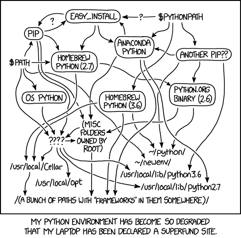
I am glad I waited to finish off this blog piece, as I found the inital set up of this a nightmare. However this really wasn’t PyXLL’s fault. I had many many python installs across different versions, both Pip and Anaconda and 32bit 3.7 and 64 bit 2.7 etc. It was awful. Reminds me of this :

Yes, my environments were a total mess too.

So I decided that as I had elected to use Anaconda for Jupyter Notebooks, I would wipe ALL of my python installs off the map and start afresh. I am super glad I did as after that all the installs and setup was miles easier and I now have a conda pyxll venv set up to play in.

Initial Python file changes

The documentation for PyXLL is very good and I was able to adapt my calc_pi code pretty easily

from random import random
from numba import njit, jit
from pyxll import xl_menu, xl_app, xlcAlert, xl_func


@xl_func
@jit
def calc_pi_numba(num_attempts: int) -> float:
    inside = 0

    for _ in range(num_attempts):
        x = random()
        y = random()

        if x ** 2 + y ** 2 <= 1:
            inside += 1

    return 4 * inside / num_attempts

@xl_func
def calc_pi_quick(num_attempts: int) -> float:
    from random import random

    inside = 0

    for _ in range(num_attempts):
        x = random()
        y = random()

        if x ** 2 + y ** 2 <= 1:
            inside += 1

    return 4 * inside / num_attempts

@xl_func
def multi_calc_pi(num_attempts: int, verbose=False) -> float:
    from multiprocessing import Pool
    from random import random
    import os
    from statistics import mean

    # lets leave one spare for OS related things so everything doesn't freeze up
    num_cpus = os.cpu_count() - 1
    # print('Num of CPUS: {}'.format(num_cpus))

    try:
        attempts_to_try_in_process = int(num_attempts / num_cpus)
        pool = Pool(num_cpus)
        # what I am trying to do here is get the calc happening over n-1 Cpus each with an even
        # split of the num_attempts. i.e. 150 attempts over 15 CPU will lead to 10 each then the mean avg
        # of the returned list being returned.
        data_outputs = pool.map(calc_pi_quick, [attempts_to_try_in_process] * num_cpus)
        return mean(data_outputs)
    finally:  # To make sure processes are closed in the end, even if errors happen
        pool.close()
        pool.join()

I did have to do some debugging which I hacked up from the examples bundled with PyXLL. Some of it was quite cool and worth noting here.

from pyxll import xl_menu, xl_app, xlcAlert, xl_func
from win32com.client import constants
import win32clipboard
import math
import time
import pydevd_pycharm


@xl_menu("Connect to PyCharm", menu="Profiling Tools")
def connect_to_pycharm():
    pydevd_pycharm.settrace('localhost',
                            port=5000,
                            suspend=False,
                            stdoutToServer=True,
                            stderrToServer=True)


@xl_menu("Time to Calculate", menu="Profiling Tools")
def time_calculation():
    """Recalculates the selected range and times how long it takes"""
    xl = xl_app()

    # switch Excel to manual calculation and disable screen updating
    orig_calc_mode = xl.Calculation
    try:
        xl.Calculation = constants.xlManual
        xl.ScreenUpdating = False

        # get the current selection
        selection = xl.Selection

        # Start the timer and calculate the range
        start_time = time.clock()
        selection.Calculate()
        end_time = time.clock()
        duration = end_time - start_time

    finally:
        # restore the original calculation mode and enable screen updating
        xl.ScreenUpdating = True
        xl.Calculation = orig_calc_mode

    win32clipboard.OpenClipboard()
    win32clipboard.EmptyClipboard()
    win32clipboard.SetClipboardText(str(duration))
    win32clipboard.CloseClipboard()

    # report the results
    xlcAlert('time taken : {}'.format(duration))

    return duration

VBA based PERFORMANCE measuring

I tried to log the performance by passing in a cell to a Python macro function in PyXLL but as PXLL support informed me if that is called from another cell, then the calculation tree is already going and it wont work. Hence I had to use a menu Item.

Then I realised that if I could get a good enough timer in VBA by hooking into some of the underlying Windows functionality I could get soe decent timing by wrapping each of the calls in a VBA call.

modTimer VBA

Type UINT64
    LowPart As Long
    HighPart As Long
End Type

Private Const BSHIFT_32 = 4294967296# ' 2 ^ 32
Private Declare PtrSafe Function QueryPerformanceCounter Lib "kernel32" (lpPerformanceCount As UINT64) As Long
Private Declare PtrSafe Function QueryPerformanceFrequency Lib "kernel32" (lpFrequency As UINT64) As Long

Global u64Start As UINT64
Global u64End As UINT64
Global u64Fqy As UINT64
 
Public Function U64Dbl(U64 As UINT64) As Double
    Dim lDbl As Double, hDbl As Double
    lDbl = U64.LowPart
    hDbl = U64.HighPart
    If lDbl < 0 Then lDbl = lDbl + BSHIFT_32
    If hDbl < 0 Then hDbl = hDbl + BSHIFT_32
    U64Dbl = lDbl + BSHIFT_32 * hDbl
End Function


Public Sub StartTimer(ByRef u64Fqy As UINT64, ByRef u64Start As UINT64)
    ' Get the counter frequency
    QueryPerformanceFrequency u64Fqy
    ' Get the counter before
    QueryPerformanceCounter u64Start
End Sub


Public Function EndTimer() As UINT64

    ' Get the counter before
    QueryPerformanceCounter u64End
    EndTimer = u64End
    
End Function


Public Function CalcTimeTaken(ByRef u64Fqy As UINT64, ByRef u64Start As UINT64) As Double
    ' User Defined Type cannot be passed ByVal and also not copying it should reduce the error seen in
    ' tioming for very small increments as we expect to see say timing something like Numba loops vs VBA for
    ' small iteations (< 1000)

    CalcTimeTaken = (U64Dbl(EndTimer) - U64Dbl(u64Start)) / U64Dbl(u64Fqy)

End Function

Wrapper VBA Function

Returns a 2 cell variant with the estimated Pi value and then the time taken

Public Function CalcPi(ByVal NumAttempts As Long, _
                       Optional ByVal CalcMethod As String = "CALCPIMONTECARLOVBA") As Variant

    Dim x(1) As Variant
    Dim StartTime As Double
    Dim EndTime As Double
    Dim TimeTaken As Double
    Dim Pi As Double
    
    
    On Error GoTo ErrHandler
    
    Pi = 0
        
    modTimer.StartTimer modTimer.u64Fqy, modTimer.u64Start
    Pi = Run(CalcMethod, NumAttempts)
    TimeTaken = CalcTimeTaken(modTimer.u64Fqy, modTimer.u64Start)
    
    x(0) = Pi
    x(1) = TimeTaken
    
    CalcPi = Application.Transpose(x)
    
    Exit Function
ErrHandler:
    Err.Raise 4444, Erl, "Error in CalcPi: " & Err.Description
End Function

Results

Performance of existing VBA – considerations

So it is interesting to note that if you have lots of small number crunching tasks to complete, moving all these to native Python might not actually save your bacon if looking for performance improvements.

CalcPiMonteCarloVBA takes almost half the time ( 24s ) vs calc_pi_quick taking 46 seconds to complete for 50,000,000 iterations.

Comparison to Jupyter Notebook

Iterations505005000500005000005000000
calc_pi_numba0.00022740.0002450.0004370.0020.01648070.1567803
calc_pi_numba Jupyter0.0000130.000020.0001610.0015880.0158830.152588
CalcPiMonteCarloVBA0.00014330.0003250.0026270.0250180.24452122.4704114
N/AN/AN/AN/AN/AN/AN/A
multi_calc_pi2.15119512.2541022.2633842.2548212.47322452.9926874
multi_calc_pi Jupyter2.8211772.8119432.7145792.7103182.9168163.315011
calc_pi_quick0.00047330.0007430.005730.048880.46228825.3454645
calc_pi_quick Jupyter0.0000710.0005040.0051170.0512970.4672264.660022

THe above table is a little data dense and not that informational but it seems that calling from PyXLL is even perhaps slightly faster than from a Notebook which is awesome news!

So computationally with Python diligence and some CompSci though we can move swathes of calculation intensive code out of VBA and into Python and get the panacea of

  • greater code control – we can assume the python code can live in a repository and have CI/CD “DevOps” practices around its delivery to the user.
  • a great library of open source functionality (pandas etc)
  • increased speed from Cython
  • code re-use (harder to do outside of XLAs)

Featured post

CALCULATE PI USING MONTECARLO SIMULATION – PHASE III – aka "Multicarlo"


Introduction

After Phase II, we discovered that Numpy wasn’t going to help. Also, getting a half way decent approximation of Pi was going to take millions of paths / attempts. So on a slimmed down calculation where the [x,y] position of each random try was not kept, what could be done to make this as quick and accurate as possible?

Multi-Processing?

Can I use the 16 Cores on my machine to go 16X faster? Am I being naiive here? If I am, how and what is the most that can be done? I would like to see if the infamous G.I.L will Get me Into Logjam or not.

First Attempt [Disaster]

from multiprocessing import Pool
import os

num_cpus = os.cpu_count()
print('Num of CPUS: {}'.format(num_cpus))

try:
    pool = Pool(num_cpus) # on 8 processors
    data_outputs = pool.map(calc_pi_quick, [10])
    print (data_outputs)
finally: # To make sure processes are closed in the end, even if errors happen
    pool.close()
    pool.join()

Disappointingly, not only is it not any quicker; in fact, doesn’t finish running AT ALL.

Awkward, lets look at why that is happening first?

  • I quite like Medium Articles and this one seems to hit the spot.
  • Also this from StackOverflow

Second Attempt

from random import random

def calc_pi_quick(num_attempts: int) -> float:
    from random import random

    inside = 0

    for _ in range(num_attempts):
        x = random()
        y = random()

        if x ** 2 + y ** 2 <= 1:
            inside += 1

    return 4 * inside / num_attempts


def multi_calc_pi(num_attempts: int, verbose=False) -> float:
    from multiprocessing import Pool
    from random import random
    import os
    from statistics import mean

    # lets leave one spare for OS related things so everything doesn't freeze up
    num_cpus = os.cpu_count() - 1
    # print('Num of CPUS: {}'.format(num_cpus))

    try:
        attempts_to_try_in_process = int(num_attempts / num_cpus)
        pool = Pool(num_cpus)
        # what I am trying to do here is get the calc happening over n-1 Cpus each with an even
        # split of the num_attempts. i.e. 150 attempts over 15 CPU will lead to 10 each then the mean avg
        # of the returned list being returned.
        data_outputs = pool.map(calc_pi_quick, [attempts_to_try_in_process] * num_cpus)
        return mean(data_outputs)
    finally:  # To make sure processes are closed in the end, even if errors happen
        pool.close()
        pool.join()

To get multiprocessing to work on Jupyter Notebooks and Windows 10, I had to save this code to a different file to be called from the Jupyter Notebook, and executed within __main__. However once I did, this did lead to a significant performance increase.

Collect the Stats

import calcpi
from timeit import default_timer as timer
from datetime import timedelta
import matplotlib.pyplot as plt

if __name__ == '__main__':
    
    num_attempts = [50, 500, 5_000, 50_000, 500_000, 5_000_000, 50_000_000]
    multi_timings = []
    single_timings = []
    
    for x in num_attempts:
    
        start = timer()
        multi_pi = calcpi.multi_calc_pi(x)
        end = timer()  
        multi_timings.append((end-start))
        print("MultiCarlo Pi: {}: {} took {}".format(multi_pi, x, timedelta(seconds=end-start)))

        start = timer()    
        pi = calcpi.calc_pi_quick(x)
        end = timer()
        single_timings.append((end-start))
        print("MonteCarlo Pi: {}: {} took {}".format(pi, x, timedelta(seconds=end-start)))

    plt.plot(num_attempts, multi_timings)
    plt.plot(num_attempts, single_timings)

    plt.show()

Display the stats in a more meaningful way

import plotly.graph_objects as go

import numpy as np

# lets pretty this up so the axis label is more readable
x_axis = ['{:,}'.format(x) for x in num_attempts]

fig = go.Figure(data=[
    go.Bar(name='Multi Process', x=x_axis, y=multi_timings),
    go.Bar(name='Single Process', x=x_axis, y=single_timings)
])
# Change the bar mode
fig.update_layout(xaxis_type='category',barmode='group')
fig.show()
Single vs Multiprocessing for increasing simulation size

Early on in the exponentially increasing simulation size, the overhead of creating the Pool, asking the os for CPU count the splitting the attempts up to the pool seemed to result in a floor of 0.4s. However, at that level the Pi value returned was nonsense anyway. So I think the overhead for any reasonable approximation of Pi is worth the set up cost in this case.

Baby, can I get your Numba?

Can we go even further? I think we could give Numba a try.

After some research and reading around the internet for a day or so while avoiding Covid-19 I found out it is incredibly simple.

4 little chars that change everything. @jit

from random import random
from numba import njit, jit

@jit
def calc_pi_numba(num_attempts: int) -> float:
    inside = 0

    for _ in range(num_attempts):
        x = random()
        y = random()

        if x ** 2 + y ** 2 <= 1:
            inside += 1

    return 4 * inside / num_attempts

That is it. Just one import and one teensy little decorator and we are away. How does this stack up agianst my mighty multi monte carlo from earlier though?

Lets get some timings

import calcpi
from timeit import default_timer as timer
from datetime import timedelta
import matplotlib.pyplot as plt
import plotly.graph_objects as go

if __name__ == '__main__':
    
    num_attempts = [50, 500, 5_000, 50_000, 500_000, 5_000_000, 50_000_000]
    function_list = [calcpi.calc_pi_quick, calcpi.calc_pi_numba, calcpi.multi_calc_pi]
    results_dict = {}

    for func in function_list:

        timings = []
        
        for x in num_attempts:
        
            start = timer()
            pi = func(x)
            end = timer()  
            timings.append((end-start))
            # print("{} => Pi: {} Attempts: {} Time: {}".format(func.__name__, pi, x, timedelta(seconds=end-start)))

        results_dict[func.__name__] = timings
    
    go_data = []
    # lets pretty this up so the axis label is more readable
    x_axis = ['{:,}'.format(x) for x in num_attempts]
    
    for func in function_list:
    
        plt.plot(num_attempts, results_dict[func.__name__])
        
        go_data.append(go.Bar(name=func.__name__, x=x_axis, y=results_dict[func.__name__]))

    plt.show()

    fig = go.Figure(data=go_data)
    # Change the bar mode
    fig.update_layout(xaxis_type='category',barmode='group')
    fig.show()
        

Results visulisation

X: Attempts Y: Seconds to run

Oh… it absolutely smashes it.

Out of the park for

  • Speed
  • Readability
  • Implementation simplicity

Featured post

CALCULATE PI USING MONTECARLO SIMULATION – PHASE II


Context

Carrying on from Phase I, I wanted to see how I could take the initial answer and make it more efficient. The first port of call then is… how expensive is it at the moment. Will any changes I make have a significant impact on that baseline.

timeit

I dont think using %%timeit as an ipython coding secret on the cell will cut the mustard, but we shall see. I would like to be able to single out code sections for timing too.

Calc Pi Unoptimised

def calc_pi(num_attempts, display_plot=False):

    import matplotlib
    import matplotlib.pyplot as plt
    from random import random
    
    inside = 0

    x_inside = []
    y_inside = []
    x_outside = []
    y_outside = []

    for _ in range(num_attempts):
        x = random()
        y = random()
        if x**2+y**2 <= 1:
            inside += 1
            x_inside.append(x)
            y_inside.append(y)
        else:
            x_outside.append(x)
            y_outside.append(y)

    pi = 4*inside/num_attempts
    
    if display_plot:
        fig, ax = plt.subplots()
        ax.set_aspect('equal')
        ax.scatter(x_inside, y_inside, color='g')
        ax.scatter(x_outside, y_outside, color='r')

    return pi

Calc Pi Quick (Version 1)

Quick Python only changes, remove array recording and if we never plan to plot remove the if statement

def calc_pi_quick(num_attempts: int):

    inside = 0

    for _ in range(num_attempts):
        x = random()
        y = random()
        if x**2+y**2 <= 1:
            inside += 1

    return 4*inside/num_attempts

Initial comparison

from timeit import default_timer as timer
from datetime import timedelta

start = timer()
calc_pi(50000000, True)
end = timer()
print(timedelta(seconds=end-start))

start = timer()
calc_pi(50000000, False)
end = timer()
print(timedelta(seconds=end-start))

start = timer()
calc_pi_quick(50000000)
end = timer()
print(timedelta(seconds=end-start))

Output

calc_pi with plotly display time: 0:00:08.318734 
calc_pi no display time: 0:00:00.625193 
calc_pi_quick time: 0:00:00.470770

We start to see there are some decent performance benefits. Lets check if these are linear or not. However to see some really decent improvements I think we can start to think about threading perhaps? Also if we still wanted to record the hit and miss positions, would numpy be quick enough that we can keep this data without a significant performance hit?

Numpy Optimisation Attempts

Spoiler Alert… my first attempt was absolutely terrible. However, in a way that’s great news. I now know what not to do with numpy on a non trivial problem, and now so do you.

def calc_pi_numpi_bad(num_attempts):
    
    import numpy as np
    import matplotlib
    import matplotlib.pyplot as plt
    from random import random
    
    inside = 0

    x_inside = np.array([])
    y_inside = np.array([])
    x_outside = np.array([])
    y_outside = np.array([])

    for _ in range(num_attempts):
        x = random()
        y = random()
        if x**2+y**2 <= 1:
            inside += 1
            x_inside = np.append(x_inside, x)
            y_inside = np.append(y_inside, y)
        else:
            x_outside = np.append(x_outside, x)
            y_outside = np.append(y_outside, y)

    pi = 4*inside/num_attempts

    return pi

How bad? Well lets see…

def measure_performance_verbose(num_attempts: int) -> None:

    from timeit import default_timer as timer
    from datetime import timedelta

    start = timer()
    calc_pi(num_attempts, False)
    end = timer()
    time_taken = end-start
    print('calc_pi time: {}'.format(timedelta(seconds=time_taken)))

    start = timer()
    calc_pi_quick(num_attempts)
    end = timer()
    quick_time_taken = end-start
    print('calc_pi_quick time: {}'.format(timedelta(seconds=quick_time_taken)))

    percentage_improvement = quick_time_taken / time_taken * 100
    
    print('Precentage improvement: {}'.format(percentage_improvement))

    start = timer()
    calc_pi_numpi(num_attempts)
    end = timer()
    numpi_time_taken = end-start
    print('calc_pi_numpi time: {}'.format(timedelta(seconds=numpi_time_taken)))
    
    start = timer()
    calc_pi_numpi_bad(num_attempts)
    end = timer()
    numpi_bad_time_taken = end-start
    print('calc_pi_numpi_bad time: {}'.format(timedelta(seconds=numpi_bad_time_taken)))
    
    
measure_performance_verbose(500_000)
calc_pi time: 0:00:00.636658
calc_pi_quick time: 0:00:00.462309
Precentage improvement: 72.6149660351135
calc_pi_numpi time: 0:00:00.616958
calc_pi_numpi_bad time: 0:12:52.784511

Whoa, what just happened there. It takes TWELVE seconds to run for 500,000 attempts. That is atrocious.

Lets look at the documentation for this function.

Ahh, that explains it. Every append copies the existing array into a new one. I did not know that, shame on me. I have always used np arrays as data converted from pandas or existing python lists, not created and appended to them on the fly.

However, we can fix it by pre-allocating the mem to the max num required and then mask the results if zero in plotly.

def calc_pi_numpi(num_attempts, display_plot=False, display_masked_plot=False):
    
    import numpy as np
    import matplotlib
    import matplotlib.pyplot as plt
    from random import random
    
    inside = 0

    x_inside = np.zeros(num_attempts)
    y_inside = np.zeros(num_attempts)
    x_outside = np.zeros(num_attempts)
    y_outside = np.zeros(num_attempts)

    for i in range(num_attempts):
        x = random()
        y = random()
        if x**2+y**2 <= 1:
            inside += 1
            x_inside[i] = x
            y_inside[i] = y
        else:
            x_outside[i] = x
            y_outside[i] = y

    if display_masked_plot:
        
        fig, ax = plt.subplots()
        ax.set_aspect('equal')
        ax.scatter(np.ma.masked_equal(x_inside,0), np.ma.masked_equal(y_inside,0), color='g')
        ax.scatter(np.ma.masked_equal(x_outside,0), np.ma.masked_equal(y_outside,0), color='r')
        
    if display_plot:
            
        x_inside2 = x_inside[x_inside !=0] 
        y_inside2 = y_inside[y_inside !=0]
        x_outside2 = x_outside[x_outside !=0]
        y_outside2 = y_outside[y_outside !=0]

        fig, ax = plt.subplots()
        ax.set_aspect('equal')
        ax.scatter(x_inside2, y_inside2, color='g')
        ax.scatter(x_outside2, y_outside2, color='r')

    pi = 4*inside/num_attempts

    return pi

There are two booleans so that we can test that both work.

calc_pi_numpi(256, True, True)
masked


numpy zero removal
start = timer()
calc_pi_numpi(500_000, True, False)
end = timer()
time_taken = end-start
print('calc_pi normal display time: {}'.format(timedelta(seconds=time_taken)))

start = timer()
calc_pi_numpi(500_000, False, True)
end = timer()
time_taken = end-start
print('calc_pi masked display time: {}'.format(timedelta(seconds=time_taken)))
calc_pi normal display time: 0:00:02.356013
calc_pi masked display time: 0:00:04.012019

Much much better.

start = timer()
calc_pi_numpi(500_000, False, False)
end = timer()
time_taken = end-start
print('calc_pi no display time: {}'.format(timedelta(seconds=time_taken)))

start = timer()
calc_pi(500_000)
end = timer()
time_taken = end-start
print('calc_pi no display time: {}'.format(timedelta(seconds=time_taken)))
calc_pi no display time: 0:00:00.622075 
calc_pi no display time: 0:00:00.655379

So… numpy doesn’t make things better, but used correctly, doesn’t make things any worse. So this is a dead end. Also we don’t want to plot for the numbers higher than a million as it looks to the human eye to be , a complete quarter circle. in plotly anyway so we dont need to store large amounts of array data anyway

While I am here I wanted to utilise the “functions are first class objects” paradigm in python. I have hinted at it by showing the initial fuction as _verbose but its much cleaner to call that same code within a functor ( of sorts ) loop as below.

def measure_performance(num_attempts: int) -> None:

    from timeit import default_timer as timer
    from datetime import timedelta
    
    funcs_to_call = [calc_pi, calc_pi_quick, calc_pi_numpi, calc_pi_numpi_bad]
    
    for func in funcs_to_call:
        start = timer()
        calc_pi(num_attempts, False)
        end = timer()
        time_taken = end-start
        print('{} time: {}'.format(func.__name__, timedelta(seconds=time_taken)))
    
measure_performance(50000)

In Phase III -> aka PiMultiCarlo I want to loo at what we can do locally on a decent multi core machine to get some decent speed improvements for only calculating the number only, not storing the guesses.

Follow-up

For Part III : CALCULATE PI USING MONTECARLO SIMULATION – PHASE III – aka “Multicarlo”

Featured post

Calculate Pi using MonteCarlo Simulation – Phase I


Context

I was interviewing for a Python developer role in an Investment bank, and a nice enough but over zealous quant started asking me silly questions. You know the sort. However in this case I didnt really know the answer. So I have determined to provide a solution I am happy that I understand and also at the same time gets me into new areas of Python development.

Question:

How would calculate the value of Pi, from scratch / first principles?

Answer I gave:

“Uhhh, pardon?

Answer I should have given:

The equation for a circle is (x-h)2 + (y-k)2 = r2. With the centre as the origin and a radius of 1 we can cancel out to : x2 + y2 ≤ 1

We then look at a quarter of the circle to take away a lot of the maths needed, and randomly insert points into the resulting square. The random, co-ords are known to be either inside or outside of the desired area. We then can get the estimation of Pi as :

We know that (Points in the circle)/(Total points) = (πr2)/(2*r)2

Which we can solve for a radius of 1 as (Points in the circle)/(Total points) = (π)/(2)2

Then π = 4 * (Points in the circle)/(Total points)

Python Implementation

Err… ok. I feel now this was quite spurious in an interview situation, but lets look at the python and see what we can do.

def calc_pi(num_attempts, display_plot=False):

    import matplotlib
    import matplotlib.pyplot as plt
    from random import random
    
    inside = 0

    x_inside = []
    y_inside = []
    x_outside = []
    y_outside = []

    for _ in range(num_attempts):
        x = random()
        y = random()
        if x**2+y**2 <= 1:
            inside += 1
            x_inside.append(x)
            y_inside.append(y)
        else:
            x_outside.append(x)
            y_outside.append(y)

    pi = 4*inside/num_attempts
    
    if display_plot:
        fig, ax = plt.subplots()
        ax.set_aspect('equal')
        ax.scatter(x_inside, y_inside, color='g')
        ax.scatter(x_outside, y_outside, color='r')

    return pi
Attempting Monte Carlo Simulation with 50 attempts. 
Pi: 3.28 

Attempting Monte Carlo Simulation with 500 attempts. 
Pi: 2.992 

Attempting Monte Carlo Simulation with 5000 attempts. 
Pi: 3.176 

Attempting Monte Carlo Simulation with 50000 attempts. 
Pi: 3.14688 

Real PI: 3.141592653589793

Plotly Visualisation

Continuing with this “interview answer” level of solution, this might make for a cool Jupyter Notebook. Lets get a graphical representation.

Lo and behold, it does! Trying with ever increasing attempts shows the quarter circle becoming more and more clear.

Monte Carlo Simulation with 50 attempts. Pi: 3.28
Monte Carlo Simulation with 500 attempts. Pi: 2.992
Monte Carlo Simulation with 5000 attempts. Pi: 3.176
Monte Carlo Simulation with 50000 attempts. Pi: 3.14688

Run Multiple times to get a mean average?

I thought that with low numbers there would be quite a large variance but the mean over multiple times would still be decent.

def plot_attempt_pi_MC_n_times(num_times, mc_attempts):

    # ok, lets use this function to try to see what the drift between that and Pi is.
    import matplotlib.pyplot as plt
    import statistics

    pi_vals = []

    for i in range(num_times):
        pi = calc_pi(mc_attempts)
        pi_vals.append(pi)

    attempt = list(range(1, num_times + 1))
    actual_pi = [math.pi]*num_times

    plt.plot(attempt, pi_vals)
    plt.plot(attempt, actual_pi)
    # a really simple arithmetic way of getting pretty close
    plt.plot(attempt, [22/7]*num_times)
    avg = statistics.mean(pi_vals)
    
    plt.plot(attempt, [avg]*num_times)
    print('Avg: {}. Diff to actual Pi: {}'.format(avg, abs(math.pi - avg)))
    plt.show()
    return pi_vals

So we can multiple times, and plot each result, then take the mean compared to the same number of attempts in one single Monte Carlo evaluation

Code to try both versions of the same number of paths

mc_pi = calc_pi(5000)
print('calc_pi(5000): {}. Diff to actual Pi: {}'.format(mc_pi, abs(math.pi - mc_pi)))
w = plot_attempt_pi_MC_n_times(100, 50)

mc_pi = calc_pi(50_000)
print('calc_pi(50_000): {}. Diff to actual Pi: {}'.format(mc_pi, abs(math.pi - mc_pi)))
x = plot_attempt_pi_MC_n_times(100, 500)

mc_pi = calc_pi(500_000)
print('calc_pi(500_000): {}. Diff to actual Pi: {}'.format(mc_pi, abs(math.pi - mc_pi)))
y = plot_attempt_pi_MC_n_times(100, 5_000)

mc_pi = calc_pi(5_000_000)
print('calc_pi((5_000_000): {}. Diff to actual Pi: {}'.format(mc_pi, abs(math.pi - mc_pi)))
z = plot_attempt_pi_MC_n_times(100, 50_000)

5,000 Attempts

calc_pi(5000): 3.1376. Diff to actual Pi: 0.003992653589793171
Avg: 3.136. Diff to actual Pi: 0.005592653589792995

50,000 Attempts

calc_pi(50_000): 3.14408. Diff to actual Pi: 0.002487346410207092
Avg: 3.14256. Diff to actual Pi: 0.000967346410206904

500,000 Attempts

calc_pi(500_000): 3.144032. Diff to actual Pi: 0.002439346410207044
Avg: 3.14292. Diff to actual Pi: 0.001327346410207042

5,000,000 Attempts

calc_pi((5_000_000): 3.1420616.
Diff to actual Pi: 0.00046894641020678307
Avg: 3.1408424.
Diff to actual Pi: 0.0007502535897931928

Conclusion

We can say without a doubt that this method of calculating Pi is both expensive AND inncaurate compared to even 22/7. This approximation only gets beaten after millions of simulation steps.

It was however an interesting foray into a number of areas of maths and Python. While it is a bit mad I would like to keep going with this. How can we make this faster locally, and what it we turned to alternative solutions like the power of the cloud to get within .. say a reliable 10dp?

Follow-up

CALCULATE PI USING MONTECARLO SIMULATION – PHASE II

Featured post

Google Music Takeout – Track Data


I always find working through a text book that it gets quite dry, and I struggle to maintain interest as the project or subject matter is too esoteric.

So, armed with a little python, StackOverflow and a search engine, I decided to see what I could do with my own data.

Photo by Clem Onojeghuo on Unsplash

What have I been listening to for the last three or four years?

Google allows users access to all their past data, and as a long time user of Google Music I wondered what the oversight on all this would be. Unlike Spotify, there doesn’t seem to be any scope for introspection into musical history or taste, which strikes me as odd. I guess Google is more about harvesting and selling the data, whereas Spotify realises that showing insight into their users activity and taste helps drive traffic and engagement levels.

Google Takeout Track dataset structure

unzipped takeout tracks, highlighting the weirder filenames

Seriously? A gazillion CSV files? Well… 14,646. That’s the best they can do? However, I then thought, hang on… combining multiple CSV files and cleaning up rubbish data in the dataset is the exact sort of basic data science 101 that every project has. Bring it on.

Track csv file combination

Python to combine the .csv files, lifted from my Jupyter Notebook

import os

# change as required, obviously
directory = '/takeout_data/Google Play Music/Tracks'

csv_files = []

for root,dirs,files in os.walk(directory):
    for file in files:
       if file.endswith(".csv"):
            csv_files.append(directory + "\\" + file)
            
print(len(csv_files))

Now lets iterate over the files found in the selected folder, add these to a list and then concatenate these into a pandas DataFrame. I’m painfully aware that the snippet below isn’t fully “pythonic” and wouldn’t win any stack overflow plaudits. However, I am backing myself to improve this at the end and I stated this would be a warts and all development blog. As such this is a “get this working to make sure I am going in the right direction and this is a good idea overall” mode. If its working I can move on and start to make enough progress to motivate myself to keep coding on the train and before bed each night. Also to be fair this code will be run on a once per archive result basis, so doesn’t need to be hugely optimised, considering the other project time dermands.

import pandas as pd

combined_csv = []
for i, csv_file in enumerate(csv_files):
    
    x = pd.read_csv(csv_file)
     
    if not pd.isna(x['Artist'].values) and x['Play Count'][0] > 0:
         if i % 100 == 0:
            print('100th Artist found: {}. Processing {}/{}'.format(x['Artist'].values, i, total))   
    
        combined_csv.append(x)

combined_df = pd.concat(combined_csv)

Which leads to the Jupyter Notebook output:

printing the output solved my “is this working?” worries

After saving this combined .csv file I thought I would have a quick peek into the data, to check what we were actually given.

Track combination sanity check

Ok, so now I know what I’ve listened to is all in one place. I now face some issues if I want to start answering the questions I had in mind.

  • Is this data reliable, how much cleaning and transformation will be needed?
  • When did these tracks get played?
  • Where can I find the metadata for this basic track info?

I created a new Jupyter notebook in order to evaluate the data. As a cursory check I thought the tthe followong would be a good test

  • See what the song length distribution was like
  • Top Artists
  • Total Number of Songs
  • DataFrame.head() displays

Jupyter Notebook : TakeoutTrackAnalysisBlog

Sorry, something went wrong. Reload?
Sorry, we cannot display this file.
Sorry, this file is invalid so it cannot be displayed.

Further questions (for another blog post)

  • What are my most popular artists, albums and genres?
  • Do I have any dirty / unknown track data
  • What are my top 10 shortest and longest tracks
Featured post

Initial foray into Data Science with Python


Professionally I have undertaken a major segue into Python from the usual Excel VBA development environment.

However this has remained very tightly linked to the quant library and specific business requirement solving as before.   So Iface the intresteing situation of nominally becoming a “Python Developer” without having the necessary interview answers or expected jobskills.

What I mean is that with Excel VBA work within Finance, and especially supporting the desks of Wholesale banks certain things are expected.   Working with Front Office designed sheets and integrating those and also the desk requirements into solutions using the IT designated strategic frameworks and technology.

So while you are expected to be very experienced / capable in Excel VBA itself it is understood that this will be back up with a large amount of esoteric and niche software across the “tech stack”.   Mainly IT developed XLAs / sheet utils and other “best practice” while using a normally mature (and highly guarded IP) layer of Quant library in some other language such as C++ / Java.

So getting things done is a case of elegantly adding in the solution to the spaghetti code thatis already there, without reinventing the wheel and / or making it any worse than it already is.    A majority of the heavy lifting on the data manipulation, trade access, market retrieval and manipulation,  valuation functionality will already be implemented bythe quant / strats function.

However the open nature of the python distribution and usage paradigm would make it insane for a bank to re invent / ignore numpy, pandas, scikit etc.   In my opinion not using the basic python libs available in Anaconda is madness.

So this leaves me with the strange situation that I am using python coupled with the quantlibrary to solve complex business problems without actually really using much of the available libraries themselves.

In effect I will be a 2 year Python developer ( on top of 12 – 15 y of financial software development ) without really being able to back that up.  Unless discussing highly proprietary Variable Annuity cases in any future project / interview.

Anyone who knows large Investment / Wholesale banking IT will know that picking up and running with some new ( to the bank ) technology and thinking isnt the done thing.  It is a configuration nightmare and makes a lot of senior people in both Front Office and also IT quite nervous.

New is bad, things should creep in slowly.   Well… Python has crept in and our small teamhas a chance to utilise most of its power as we see fit.   So I plan to familiarise myself with the Data Science elements via extra curricular development and hope that keeps my CV sharp while also providing a chance to try something interesting.

Featured post

Google Takeout – Music Activity Data


After looking through the Takeout data for the tracks I have listened to I cannot see any sort of unique ref for track, artist or album. There isn’t any id on the .csv file itself. Uh oh. I realised this was super gross. None of the data would be linked to the actual track ids etc.

Photo by Martijn Baudoin on Unsplash

This is fine for skilling up for some Data Science techniques, but otherwise? Unless I am getting something seriously wrong here Google have really dropped the ball on interlinking their data here… I mean, its GOOGLE right?

I scratched around and found that a sub section of Google Activity would help on the when, and applied for the archive. Surely this would be better and all would be revealed?

lets deselect all the other guff right now as that is pointless work to wade through later for a few clicks now

At first I got the wrong format, as I intended to use pandas.DataFrame functions so I’d be better off in JSON for the starting point.

when working with pandas JSON is much much easier than a mess of HTML

Lets have a look at this JSON via a Jupyter Notebook display on head and see what we can determine

import requests
import json
import pandas as pd
from pandas.io.json import json_normalize 
r = requests.get(r'https://raw.githubusercontent.com/FinancialRADDeveloper/GoogleMusicDataAnalysis/master/takeout_data/My%20Activity/Google%20Play%20Music/My%20Activity.json')
activity_data_frame = json_normalize(r.json())

display(activity_data_frame.head())

This isn’t good news either. WTAF Google, how is anyone supposed to use this data?

WTAFactivity dataframe head()

Ok, so it is just as bad for interlinking as it was for track data. I’m kicking myself for not using Spotify premium a few years ago! Maybe I’m missing something but the Spotofy API is littered with URIs and other data to link everything together, whereas with Google Music I’m left with the option scrabbling around with text parsing? However, while annoying, it is perfect for skilling up on some data science basics.

This leaves some questions we need to answer:

  • Can we do data verification between the tracks listened to, and the Google Music activity?
  • What does the general total and daily activity look like?
    • How should I display this?
  • Can I display meaning ful stats on most popular choice per hour of the day?

I think any further analysis will start to need to delve into some more Meta data, which will be covered in another post regarding web scraping or Spofy API via spotipy.

Listening stats per hour

import matplotlib.pyplot as plt

plt.ion()
plt.bar([i[0] for i in daily_listening_stats], [j[1] for j in daily_listening_stats], color = 'blue')
plt.bar([i[0] for i in skipped_stats], [j[1] for j in skipped_stats], color='red')
plt.bar([i[0] for i in search_stats], [j[1] for j in search_stats], color='purple')
plt.xlabel('Hour of the Day')
plt.ylabel('Total tracks')

plt.show()

This seems roughly in line with expectations. Some late at night then a big dip while asleep and then a ramp up. I do’t tend to listen much on the commute, but will listen to something at the start of the working day. Then a dip for lunch, and some listening from then till tailing down on the eveing when eating or watching TV with my wife.

Daily Listening Stats:

import requests
import json
import pandas as pd
from pandas.io.json import json_normalize 
import matplotlib.pyplot as plt


r = requests.get(r'https://raw.githubusercontent.com/FinancialRADDeveloper/GoogleMusicDataAnalysis/master/takeout_data/My%20Activity/Google%20Play%20Music/My%20Activity.json')
activity_data_frame = json_normalize(r.json())

listened_to_dataframe = activity_data_frame[activity_data_frame['title'].str.contains("Listened to")]

display(listened_to_dataframe.sample(10))

listened_to_dataframe['activity_datetime'] = pd.to_datetime(listened_to_dataframe['time']).copy()

daily_stats = listened_to_dataframe['activity_datetime'].dt.date.value_counts()
daily_stats_sorted = daily_stats.sort_values(ascending=True)
daily_stats_sorted.plot(legend=True)

Further analysis and visualisation

It would be really interesting to get into the meta data.. I can work out my favourite tracks and artists per hour of the day but its going to be much harder to work out styles or genres. As mentioned before it should force me to go and learn another area of Data Science and python though.

Cross Validation

If each track entry has a ‘Play Count’ field, can I safely assume that if i pick out a sample of tracks, I’ll be able to find the correct Activity entries? Let us see shall we. I’ll take some of the most popular tracks, as a few missed listens should matter alot less.

Foray Into Data Science – Part II


As mentioned in my earlier article, I am starting to get into Data Science. I might be quite late to the party in some respects but better late then never I guess.

https://financialraddeveloper.com/2019/09/01/initial-foray-into-data-science-with-python/

Building from my intial thoughts and ideas I thought I would go throug the process, as I experienced it, in a series of posts here. I often read highly polished “how to” articles but I would like to include a warts and all journey through all the obstacles / sticking points and general quagmire of head scratching and confusion that people (maybe it is just me) experience when starting out something new.

To be honest even restarting / setting up this blog after a significant haitus was a > 1hr chore I wasn’t expecting. Even then I am not sure if the WordPress.exe is worth the time or RAM it sucks in.

Equipment:

This shaped quite a bit of my decisions later on down the line so I will state what I have, so that those calls don’t look so odd later on.

The ASUS Powerbook tablet combo was a few hundred quid back in 2015 but my wife didn’t like it, and so I dusted it off after a colleague intrigued me with his much fancier Windows Surface Pro style laptop. For the < £150 that it can be purchased for now it is a total bargain, especially with the ability to put a memory card in the tablet part and having a 500Gb HDD in the keyboard. As I reckon I cannot realistically develop any meaningful Python without a half decent keyboard ( and certainly not an on screen one ) I installed the PyCharm and Anaconda parts to the E: drive that comes up when the unit is “complete”.

One nice side effect is that I have to really consider performance and efficiency when I am both developing and also in my own environment. Which explains my early doors switch away from PyCharm and into Spyder and Jupyter Notebooks. The overhead of the Java based Eclipse part of PyCharm caused my morning train development to really slow to a crawl.

On a side note I got a great deal on my HP Z600 Workstation which until my clients switch to Win 10 a clone of my professional development workstation

This will be reclaimed old stock from somewhere but I love a bargain and the idea of getting that much RAM and CPU for under £500 when some company probably specced that bad boy 5+ years ago for £5k makes me very happy.

The Death of IT Contracting? – IR35 6th April 2020 – Off Payroll Rules impact


Private sector IR35 Off-payroll working rules are coming, the best way to be informed is straight from the horses mouth:

https://www.gov.uk/guidance/april-2020-changes-to-off-payroll-working-for-intermediaries

After many failed attempts by HMRC, it seems like they are going to kill off Ltd company contracting. I can already hear grumbling and dissention at the back but I think you should hear me out. I think this will happen unintentionally via the back door. I dont think this is an actual witch hunt, more of a incorrectly judged tax grab / “equalisation” attempt which will spectacularly backfire.

The actual stats and or verified links to hard evidence seem quite thin on the ground. However, from my own experience and research it seems that HMRC has investigative capacity for around 250 reviews per year. Included in the following link is a very useful history of IR35 cases and significant occurences and changes:

https://www.contractorcalculator.co.uk/ir35_history.aspx

Of those it seems like they are only successful with a very very small number of them. Often trying and failing to pick a high profile example (often inexplicably a popular and innocent seeming celebrity) and then failing to prove their own standards and rules with any coherence. Ignoring their own tool when it suits them and never quite coing to a set of definitive practices and rulings.

Considering this, it could have been sensible to drop the whole mess and accept that tax avoidance not evasion, occurs in many places and publicly letting off big firms such as Vodafone, Goldman Sachs and Boots etc every year for billions of pounds while chasing the little man PSC seems a little odd.

However some sneaky genius seems to have worked out that if they take on who is responsible for payment of tax and declaring in or out from the end company ( us contractors) and reverse the order of chasing debt and responsibility then they might have more luck.

At first I thought this might be great news. Previously, contract review and trying to engage clients ( especially large London based financial instituions) in correct IR35 friendly practices has always been an uphill battle. A few issues contractors face:

  • Timesheets
    • Billing is in day rate and there should be a project scope
  • Reporting lines, being assigned a “manager” who is far too junior
  • Not being assigned project based work
    • Support Rotas , BAU tasks and ever changing requirements set daily and arcing over multiple workstreams unrelated to the inital project terms.
  • Appearing on org-charts
  • Being compelled to embark on compliance / company wide training marked “mandatory for all EMPLOYEES”
  • Work email addresses

Essentially clients give contractors the stuff of nightmares under the Control section of the “caught by IR35” guideline. This would have never changed as the client often views the engagement as another role, a seat with a human from another budget. For far too long the clients have been filling roles, conducting interviews, assessing team fit. All this is nonsense in the eyes of the legislation and is so common place / rife in the contracting world it has become a crazy sort of normal.

Well, thats not going to happen any more. Now that the justification / CEST checking etc lands squarely with the end client and they are on hook for multiple contractors being caught at once and being landed with a large bill, unsuprisingly they are starting to treat the engagement process and working practices with some actual rigour. Rigour that was deserved all along. As seen in 2008 Financial crises and a further smorgasbord of poor behaviour and a litany of dubious practices, clients ( such as financial institutions) et al will always do the minimum needed until regulated to do something else.

We already see some Banks in London declaring this basically too much of a headache to sort out and laying down an official policy to remove all Ltd Co PSC contractors before April 2020 or getting CXO office approval for any remaining needs. How hypocritical is this? Its fine until you are on the line for investigation, then your internal legal team and HR have a look and decide to do it properly will be a bit complicated and so bin it all off?

https://www.larsenhowie.co.uk/knowledgehub/hsbc-cull-contractors-ir35

Have you ever noticed how this will have an impact to a large section of a certaintype of worker in an industry leaidng them, all to be in effectlaid off all at the same time? What like Miners or Steel workers… Nary a tear shed for hundreds to thousands of IT contractors though! Go figure.

So what options are we left with?

https://news.efinancialcareers.com/uk-en/3001526/contractor-job-market-banking

  • Move to Fixed Term Contract as PAYE direct with clients
  • Be declared as “In” and the bank extracts the Employers NI and PAYE etc at source
    • Will rates be increased to compensate for this? Will clients try to keep their costs the same and pass this through unapologetically?
    • Pressure exerted during the turmoil to accept being essentially perm with none of the benefits, job security, progression and training. Will they offer and acceptable uplift to compensate for this?
  • Move over to perm at some HR computed rate
    • Does this have any retrospective implications for previous contract work at the client
    • Will the rate be commensurate with the levekl of income expected by the contractor for a similar amount of work / time spent at the client?
    • How will the client themselves react to the budgetary pressure placed on the different departments with increared perm worker overhead, benefits etc
  • Continue in an “Out” contract
    • Will this still be the same contractas before. If the legal team deem certain areas need to be re specified, i.e.HMRC CEST compliance changes are required, what happens to the status of the contracts before , if any were engaged? Do these look more “In” than before

These leaves me with the final question, what dothe contractors themselves in the provate sector plan to do? Some will be IR35 Public secotr reform refugees and some will be long term contractors, which have avoided the perm games / required responsibilities that are lumped into Senior Developer roles such as reporting lines, budgeting etc.

Quick Transposer


A post from a Pistonhead member in need :

Hopefully someone can help!

I have a list of approx 50000 numbers in ‘Column A’ of spreadsheet. I need to split this list into batches of 1000, populated into Column B onwards.

Anyone with some VBA skill got any ideas? Thanks in advance!

 
My reply :
 
Sub QuickTranspose()

    Dim rng As Range
    Dim StartRowNum As Long
    Dim EndRowNum As Long
    Dim ColumnOffsetCounter As Long
    Dim GroupSize As Long
    Dim v
    Dim i As Long
    Dim TotalRows As Long
    GroupSize = 1000
    TotalRows = 50000
    
    'Dirty but without range names etc you just need to get the
    'selected cell to be the first one in the list
    Set rng = Application.Selection
    StartRowNum = rng.Rows.Row
    For i = 0 To TotalRows / GroupSize
        EndRowNum = StartRowNum + GroupSize - 1
        v = Range("A" & StartRowNum & ":A" & EndRowNum).Value
        Range(rng.Offset(0, i + 1), rng.Offset(GroupSize - 1, i + 1)).Value = v
        StartRowNum = EndRowNum + 1
    
    Next i
End Sub

Blog at WordPress.com.

Up ↑